Convolutional Neural Network (CNN) – Backward Propagation of the Pooling Layers

There is a myriad of resources to explain the backward propagation of the most popular layers of neural networks for classifier problems, such as linear layers, Softmax, Cross Entropy, and Sigmoid. However, it is much less common to see resources for backward propagation for the convolutional neural network (CNN). Most deep learning resources introduce only the forward propagation for CNN, and leave the part of backward propagation for high level deep learning frameworks, such as TensorFlow or Keras, to worry about.

I am going to provide some quick visualizations of how to deal with the backward propagation for average pooling and maximum pooling layers of the CNN network in this post. For the sake of simplicity, I would use the filter with (height, width, stride) = (3, 3, 1) (i.e. we would not care about padding as we would just look at a partial area). We would be doing this in the Numpy library environment (of Python 3), as we are looking at the low level structures.

The average pooling layer was popular before the rise of maximum pooling layer in the 00s. The original LeNet-5, one of the pioneer CNNs in the 90s, is in fact using an average pooling layer after each convolution layers. The maximum pooling layer, in contrast, is relatively new. It is able to capture the features of the output of previous layers even more effectively than the average pooling layer, and is, unsurprisingly, more popular in modern CNN.

Backward propagation of Average Pooling Layer

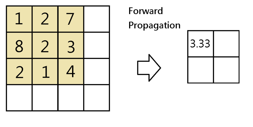
As you may know, average pooling layer takes the average of the values being scanned by the filters. Therefore, for each scanning index , , filter size  and output , we have:-

Please note that m is the m-th data point of the mini batch, while c is the c-th channel. Below is an illustration of when is taken as :-

Forward propagation of the average pooling layer with filter size (3, 3) in one scan.

Therefore, for backward propagation, in finding out partial derivatives (i.e. the components of the matrix ), we can see that each of them contributes to  of the output (components of the matrix ) in each scan. Thus we can distribute back the derivatives  to the previous layer by chain rule, as below:-

Backward propagation of the average pooling layer. Figures on the right are the respective values of dA of the current layer. The above gif focuses on the yellow cell for illustration purpose. In fact, the mean of derivatives would be added to all nine cells within the grey grid at the left in every moves.

To do it in Numpy, given dA, we would obtain dA_prev by running the below code for all i and j:-

import numpy as np
average_dA=dA[m,i,j,c]/H/W
dA_prev[m, i:(i+H), j:(j+W), c] += np.ones((H,W))*average_dA

Backward propagation of Maximum Pooling Layer

The maximum pooling layer takes only the maximum number of the values being scanned by the filter. That is:-

Forward propagation of the maximum pooling layer with filter size (3, 3).

Since only the maximum value would impact the respective cell of the next layer, , the backward propagation would only apply to those that have maximum value in each move:-

Backward propagation of maximum pooling layer. The figures at right are the dA (large font) and A (small font) of the current layer. The red spot demonstrates the cell with largest value within the filter.

To do it in Numpy, we would apply a mask to the dA as belowfor all i and j:-

a_prev_slice = a_prev[vert_start:vert_end,horiz_start:horiz_end,c]
mask = (a_prev_slice==np.max(a_prev_slice))
dA_prev[m, i:(i+H), j:(j+K), c] += mask*dA[m,i,j,c]

Backward propagation of Convolution Layer, and conclusion

Another blogger, Mayank Agarwal, had written about the backward propagation of convolution layer with clear illustration. Understanding the backward propagation of the pooling layer would make backward propagation of the convolution layer a lot less complicated.

As we can see, the formulation of the backward propagation of the pooling layer may involve lots of notation (since data points, height, width, channels would form a rank-4 tensor) and have clumsy mathematical representation as the forward propagation involves partial operations in space, but that is not complicated in intuition.